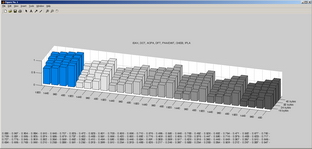
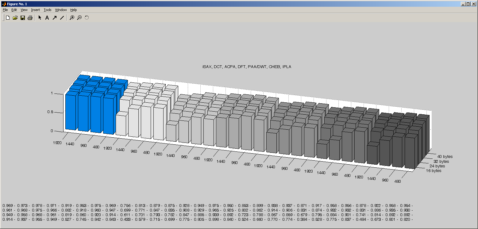
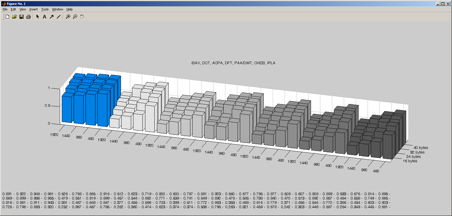
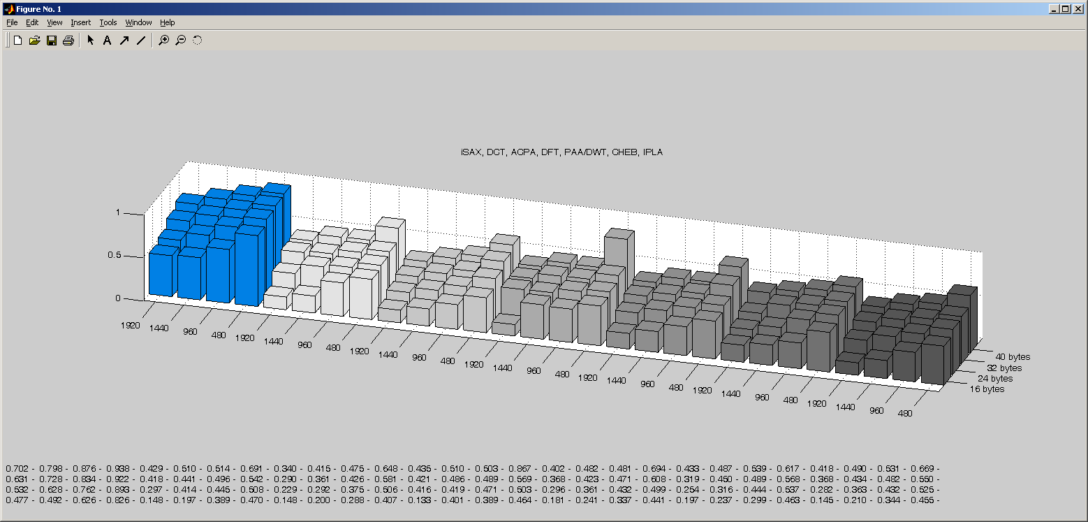
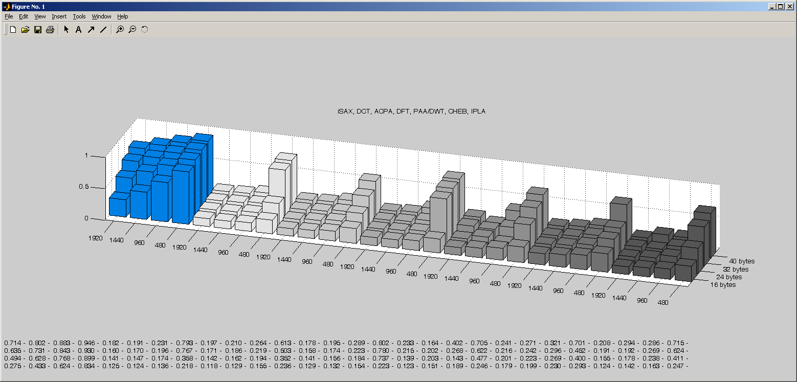
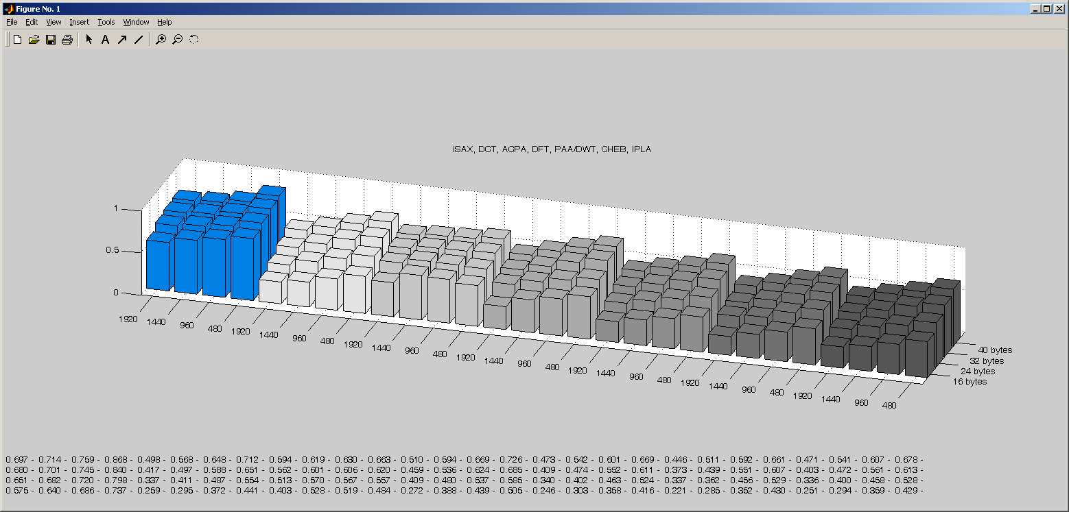
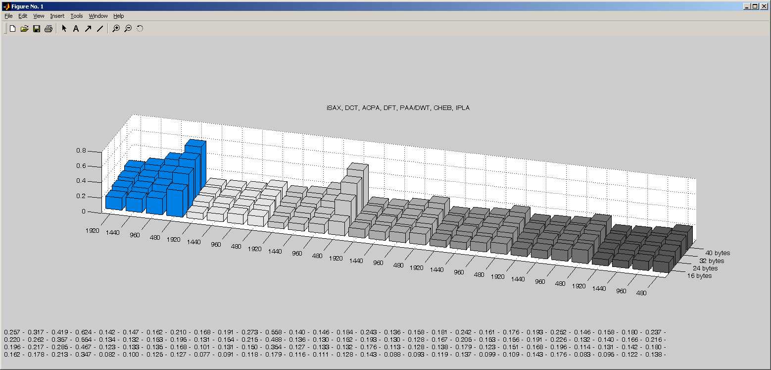
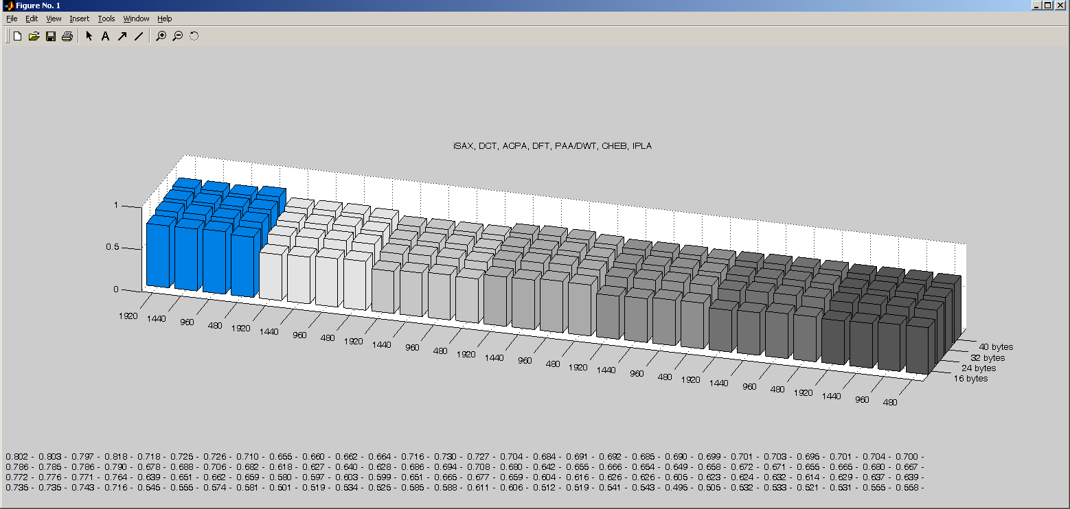
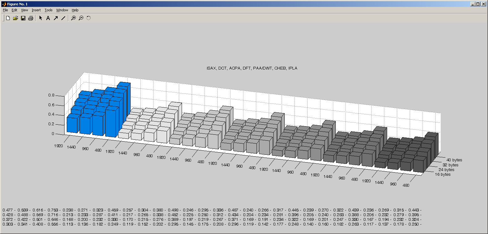
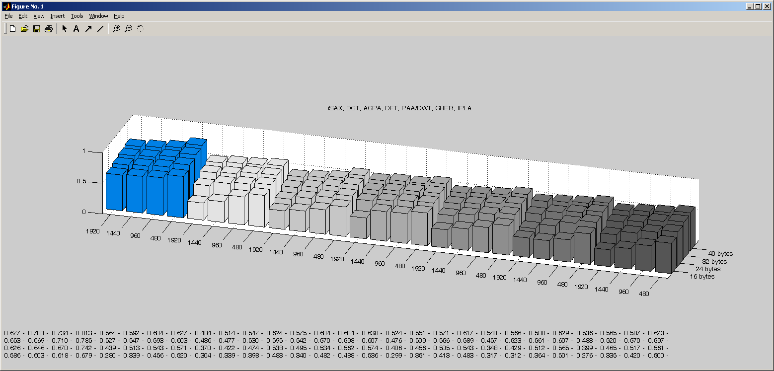
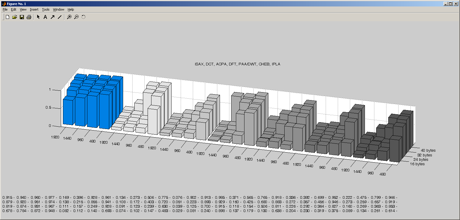
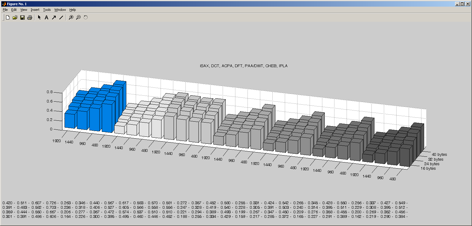
Here we consider T, the tightness of lower bounds. This is calculated as:
T = LowerBoundDist(a,b) / TrueEuclidianDist(a,b)
We randomly sample a and b (with replacement) 1,000 times for each combination of parameters. We vary the time series length [480, 960, 1440, 1920] and the number of bytes available per time series [16, 24, 32, 40]. We assume that each real valued representation requires 4 bytes per coefficient thus they use [4, 6, 8, 10] coefficients. For iSAX, we hard code the cardinality to 256, and we thus have [16, 24, 32, 40] words. For each experiment we created a bar chart and table. In addition, we include a link to the dataset if the dataset is not already in the public domain (UCR Archive data is here, warning 500meg file, password peggy).
Recall that larger values are better. If the value of T is zero, then any indexing technique is condemned to retrieving every object from the disk. If the value of T is one, then there is no search, we could simply retrieve one file from disk and guarantee that we we had the true nearest neighbor. Note that the speedup obtained is generally non-linear in T, that is to say if one representation has a lower bound that is twice as large as another, we can usually expect a much greater than two-fold decrease in disk accesses.
- Pen: Image, Original Time Series Data. Data came from this paper: Behzad Malek, Mauricio Orozco and Abdulmotaleb El Saddik "Novel Shoulder-Surfing Resistant Haptic-based Graphical Password" Proc. of the EuroHaptics 2006 conference, July 3-6 Paris, France.
- Koski ECG: Image, Original Time Series Data. Data came from this paper: Antti Koski: Primitive coding of structural ECG features. Pattern Recognition Letters 17(11): 1215-1222 (1996)
- Steamgen: Image, Original Time Series Data. Data came from this paper: G. Pellegrinetti and J. Benstman, Nonlinear Control Oriented Boiler Modeling -A Benchmark Problem for Controller Design, IEEE Tran. Control Systems Tech. Vol.4No.1 Jan.1996
- Star Light Curve Image, Original Time Series Data. Data came from Harvard University Time Series Center.
- Mallet: Image, Original Time Series Data is in UCR Archive (here, warning 500meg file). Data came from this paper: M. K. Jeong, J. C. Lu, X. Huo, B. Vidakovic, and D. Chen (2006), "Wavelet-based Data Reduction Techniques for Process Fault Detection," Technometrics, 48(1), 26-40
- Power_Data : Image, Original Time Series Data is in UCR Archive (here, warning 500meg file). Data came from this paper: van Wijk J. J. and van Selow E. R. Cluster and calendarbased visualization of time series data. In Proc. IEEE INFOVIS, pages 4-9, Oct. 25-26, 1999.
- Clorine (cl2fullLarge) Image: Original Time Series Data. Data comes from this website.
- Kung Fu MoCap: Image, Original Time Series Data. Data comes from this paper.
- PostureCentroidB Image, Original Time Series Data. Data comes from Jessica Lin, Eamonn J. Keogh, Stefano Lonardi, Jeffrey P. Lankford, Donna M. Nystrom: Visually mining and monitoring massive time series. KDD 2004: 460-469, see fig 13, 15.
- Ann_gun_CentroidA Image, Original Time Series Data. Data comes from Ratanamahatana, C. A. and Keogh. E. (2004). Making Time-series Classification More Accurate Using Learned Constraints. SDM '04 see fig 8
- Converted_ERP Image, Original Time Series Data. Data comes from this paper.
- Tickwise Image, Original Time Series Data. Data comes from here.
- Foetal_ecg Image, Original Time Series Data is in UCR Archive (here, warning 500meg file) L. De Lathauwer, B. De Moor, J. Vandewalle, Fetal Electrocardiogram Extraction by Source Subspace Separation. Proc. IEEE SP / ATHOS Workshop on HOS, 1995.
- Buoy Sensor Image, Original Time Series Data is in UCR Archive (here, warning 500meg file) The Center for Coastal Studies' Data Zoo.
- Winding Image, Original Time Series Data is in UCR Archive (here, warning 500meg file) This is one of the DaISy datasets.
- CSTR Image, Original Time Series Data is in UCR Archive (here, warning 500meg file) This is one of the DaISy datasets.
- Burst Image, Original Time Series Data is in UCR Archive (here, warning 500meg file) This is one of the DaISy datasets.
- Fluid_dynamics Image, Original Time Series Data is in UCR Archive (here, warning 500meg file) Data comes from, Garabadu, Thompson, Lindstrom and Klewicki (2003). Fast and Accurate NN Approach for Multi-Event Annotation of Time Series . UUCS-03-021.
- Tide Image, Original Time Series Data is in UCR Archive (here, warning 500meg file). From paper: Analysis of Subtidal Coastal Sea Level Fluctuations Using Wavelets" by D. B. Percival and H. O. Mofjeld, JASA September 1997, Vol. 92, No. 439, 868-880.
- Motorcurrent Image, Original Time Series Data is in UCR Archive (here, warning 500meg file) From papers of Richard J. Povinelli.
- Muscle Activation Image, Original Time Series Data is in UCR Archive (here, warning 500meg file) From Hoos, O., Department of Sports Medicine, Philipps-University Marburg, Germany Morchen, F., Department of Mathematics and Computer Science, Philipps-University Marburg, Germany
- Physiodata (npo141) Image, Original Time Series Data is in UCR Archive (here, warning 500meg file)
- Respiration Image, Original Time Series Data is here, as used in E. Keogh, J. Lin and A. Fu (2005). HOT SAX: Efficiently Finding the Most Unusual Time Series Subsequence (ICDM 2005)
- ECG (mitdbx_mitdbx_108) Image, Original Time Series Data is here, as used in E. Keogh, J. Lin and A. Fu (2005). HOT SAX: Efficiently Finding the Most Unusual Time Series Subsequence (ICDM 2005)
- ECG (chfdb_chf01_275) Image, Original Time Series Data is here, as used in E. Keogh, J. Lin and A. Fu (2005). HOT SAX: Efficiently Finding the Most Unusual Time Series Subsequence (ICDM 2005)
- TOR( Italy power demand 97 Image, Original Time Series Data is in UCR Archive (here, warning 500meg file)
- Trajectory3_7_2006.bmp Image, Original Time Series Data is in UCR Archive (here, warning 500meg file) From this paper: Pokrajac, Lazarevic, Latecki: Incremental Local Outlier Detection for Data Streams. CIDM 2007: 504-515
- Synthetic Lightning EMP Image, Data and explanation is here. Synthetic Lightning EMP Classification Data Sets
- Lightning (forte6class) Image, Data and explanation is here. FORTE Time Series Classification Data Sets.
.bmp)
.bmp)
.bmp)
.bmp)
.bmp)
.bmp)
.bmp)
Notes:
-
There is an apparent paradox in the some datasets, including Muscle Activation dataset. The tightest of the lower bounds improves from 480 to 960. How is this possible? The data consist of noisy steps, like this [1, 2, 0, 1, 2, 0, 101, 100, 101, 103, 100, 0, 1, 2, 1, ...]. If a subsequence straddles at least one step, then the representation devotes most of its energy in approximating that step. However, if the subsequence falls within a single step, the z-normalization "expands" the signal to pure noise, which is hard to approximate. In this case, only the subsequences of length 480 can fall within a single step.
-
In general, there is little difference between DCT, DFT, PAA, iPLA and CHEB. This has been noted before (see table 1 of this paper). APCA is slightly worse that the rest if the data is completely stationary, but can be significantly better on datasets that are bursty, see Synthetic Lightning EMP as an example. Note that this dataset exhibits the apparent paradox discussed above. The Foetal_ecg dataset also exhibits this burstyness and corresponding improvement for APCA.
Here is a spreadsheet which contains the raw numbers for the SAX vs PAA experiment in Figure 4 of the paper. The raw time series data is here. In the zip there are two files ts1.txt and ts2.txt (each line in each file represents a normalized time series of length 256, there should be 10,000 lines each). For each run of the experiment we require two time series, this corresponds to an entry in ts1.txt and an entry in ts2.txt. i.e. line 4 in ts1.txt is paired with line 4 in ts2.txt
The Contig NT_005334.15 of human chromosome 2 is here (Local version here). Below in blue (human) and red (chimp) are the two similar sequences plotted in the paper.
GTCAATGGCCAGGATATTAGAACAGTACTCTGTGAACCCTATTTATGGTGGCACCCCTTAGACTAAGATAACACAGGGAGCAAGAGGTTGACAGGAAAGCCAGGGGAGCAGGGAAGCCTCCTGTAAAGAGAGAAGTGCTAAGTCTCCTTTCTAAGGCACATGATGGAT
TCAAGGGAAAGCCACATTTGACTAAAGCCCAAGGGATTGTTGCTTCTAATCCGATTTCTTGGCAGAAGATATTACAAACTAAGAGTCAGATTAATATGTGGGTGCCAAAATAAATAAACAAATAATTGAATAATCCCTGGAGGTTTAAGTGAGGAGAAACTCCTCCAC
AGCTTGCTACCGAGGCAGAACCGGTTGAAACTGAAATGCATCCGCCGCCAGAGGATCTGTAAAAGAGAGGTTGTTACGAAACTGGCAACTGCCAACCAAAGTCCACCAATGGACAAGCAAAAAAGAGCACTCATCTCATGCTCCCAAGGATCAACCTTCCCAGAGTTT
TCACTTAAGTGGCCACCAAGCCAGTTGTCAATCCAGGGCTTTGGACTGAAATCTAGGGCTTCATCCGCTACCTCAGAGTGTCTTCTATTTCTTCCAGCCAGTGACAAATACAACAAACATCTGAGATGTTTTAGCTATAAATCCTTTACAATTGTTATTTATGTCTTA
ACTTTTGTTATACCTGGAAAAGTAGGGGAAACAATAAGAACATACTGTCTTGGCCAAGCATCCAAGGTTAAATGAGTTATGGAAATTCATTTGGGAGCCAAGACATTGCACGTGGTTATTTATTAGTCACCCAAGCATGTATTTTGCATGTCCATCAGTTGTTCTTGG
CCAAAAGAGCAGAATCAATGAGCCGCTGCAGATGCAGACATAGCAGCCCCTTGCAGGGACAAGTCTGCAAGATGAGCATTGAAGAGGATGCACAAGCCCGGTAGCCCGGGAAATGGCAGGCACTTACAAGAGCCCAGGTTGTTGCCATGTTTGTTTTTGCAACTTGTC
TATTTAAAGAGATTTG
GGCAATGGCCAGGATATTAGAACAGTACTCTGTGAACCCTATTTATGGTAGCACCCCTTAGACTAAGATAACACAGGGAGCAAGAGGTTGACAGGAAAGCCAGGGGAGCAGGGAAGCCTCCTGTAAAGAGAGAAGTGCTAAGTCTCCTTTCTAAGGCACATGATGGAT
TCAAGGGAAAGTCACATTTGACTAAAGCCCAAGGGATTGTTGCTTCTAATCCGATTCTTGGCAGAAGATATTGCAAACTAAGAGTCAGATTAATATGTGGGTGCCAAAATAAATAAACAAATAATTGAATAATCCCTGGAGGTTTAAGTGAGGAGAAACTCCTCCACA
GCTTGCTACCGAGGCAGAACCGGTTGAAACTGAAATGCACCCGCTGCCAGAGGATCTGTAAAAGGGAGGTTGTTACCGAACTGGCAACTGCCAACCAAAGTCTACCAATGGACAAGCAAAAAAGAGCACTCATCTCATGCTCCCAAGGATCAACCTTCCCAGAATTTT
CACTTAAGTGGCCACCAAGCCAGTTGTCAATCCAGGGCTTTGGACTGAAATCTAGGGCTTCATCCACTACCTCAGAGTGTCTTCCATTTCTTCCAGCCAGTGACAAATACAACAAACATCTGAGATGTTTTAGCTATAAATCCTTTACAATTGTTATTTATGTCTTAA
CTTTTGTTATACCTGGAAAAGTAGGGGAAACAATAAGAACATACTGTCTTGGCCAAGCATCCAAGGTTAAATGAGTTATGGGAATTCATTTGGGAGCCAAGACATTGCGCGTGGTTATTTATTAGTCACCCAAGCATGTATTTTGCATGTCCATCAGTTGTTCTTGGC
CAAAAGAACAGAATCAATGAGCCGCTGCAGATGCAGACATAGCAGCCCCTTGCAGGAACAAGTCTGCAAGATGAGCATTGAAGAGGATGCACAAGCCCGGTAGCCCGGGAAATGGCAGGCACTTACAAGAGCCCAGGTTGTTGCCATGTTTGTTTTTGCAACTTGTCT
ATTTAAACAGATTTGA
Due to space limitations, we did not show the effect of changing the parameters th, or w. We do this here. First read the readme file, then w is addressed here and th is addressed here.