
This data contains tongue and lip time-series movement data in producing 25 words collected from multiple speakers of native English. Electromagnetic Articulograph was used to collect the data, where small wired sensors were attached on the surface of tongue and lips.
Each data file is a sample (example) - production of a word, by one speaker.
The data files have been segmented (from long sequences) into individual words, which means the beginning of a data file is the beginning of a word production, the end of the data file if the end of the word production.
12 sensors were used for data collection, including HC, HL, HR, T1, T2, T3, T4, UL, LL, JC, JL, and JR.
HC, HL, HR are head sensors; T1 - T4 are tongue sensors, from tongue tip to tongue back in the midline;
UL and LL are lip sensors; JC, JL, and JR are jaw sensors;
Data from head sensors are used for calculating head-independent movement of other sensors.
The validity of jaw sensor data is not verified. Thus, currently, only tongue and lip data are available for word classification.
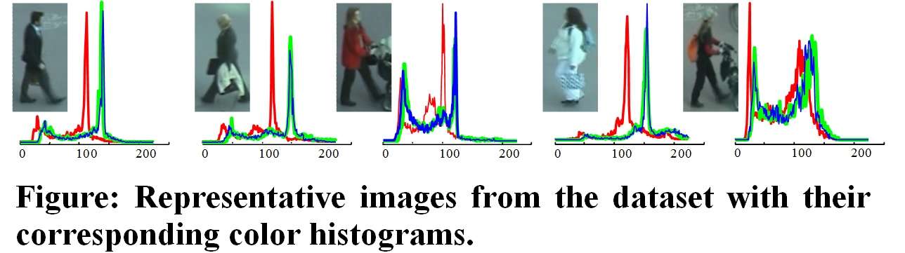
In our experiment we used data from the lower lip sensor. We preprocessed the data to contain 18 different words.
Data
For any data related question, contact (Dr. Jun Wang)
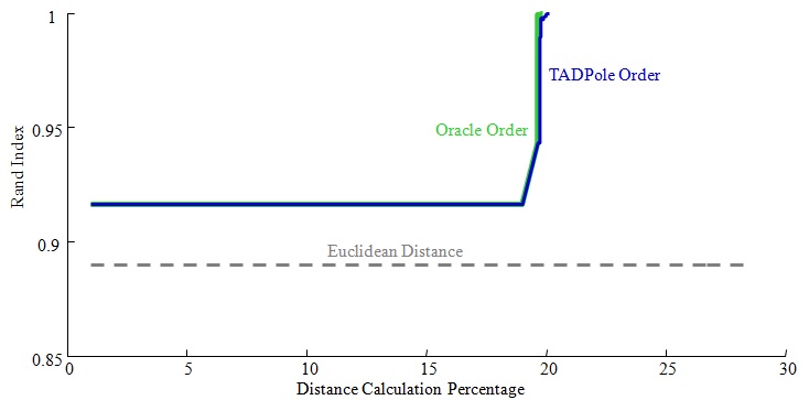
Anytime Experiment
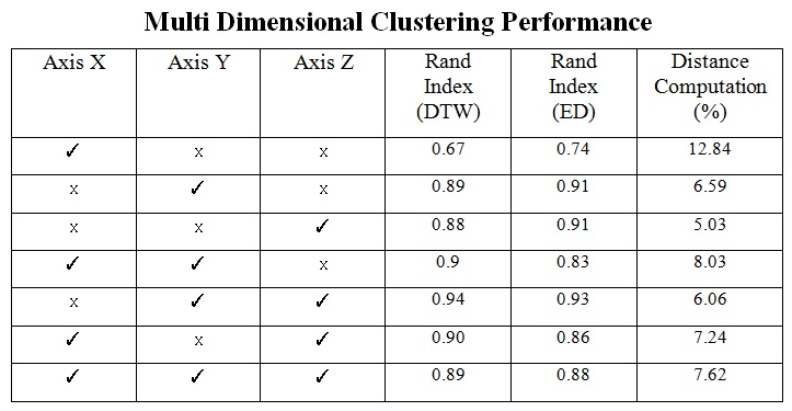
We demonstrate the accelerated multi dimensional clustering problem under DTW in the Table below.
As we can see, using a single axis to do the clustering does not give the best results (row 1-3).
In addition, using all the axes is useful neither (row 8). However, if we carefully omit irrelevant axis
(in our case it is X axis, because it is only useful for patients with facial asymmetry), then we can perform very well in terms of cluster quality, and distance computation (row 5).
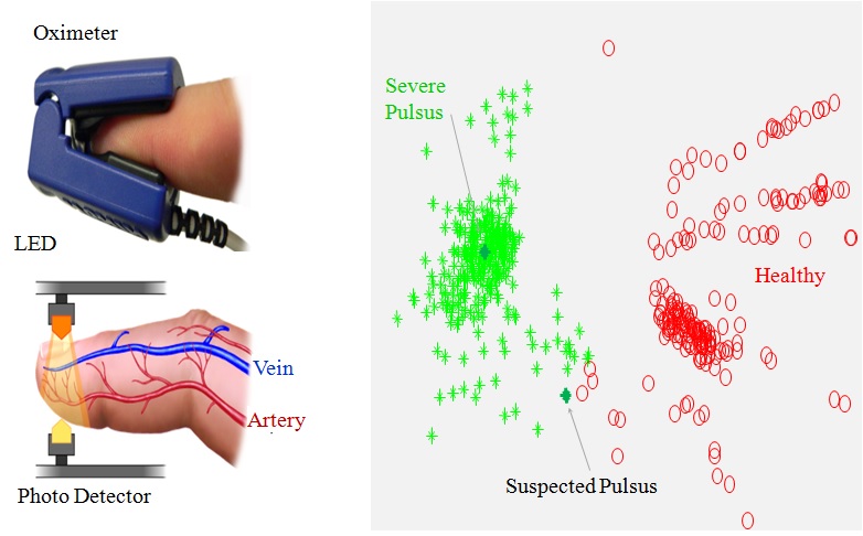
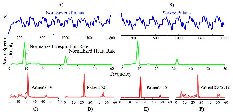
Pulsus Paradoxus is defined as a significant decline in the pulse with inspiration.
It is a symptom of Cardiac Tamponade, a life-threatening condition where high-pressure fluid fills the sac surrounding the heart.
Of the several ways to detect Pulsus, the least invasive and simplest uses the PPG (PhotoPlethysmoGram).
In the figure below we show the PPG measurement process. From the right figure, we can see that the Pulsus instances are within a compact cluster,
and the non-Pulsus instances seem to form a number of sub-clusters. Our medical collaborator suggests this reflects the fact that there is one way to have Tamponade, but multiple ways to have a healthy heartbeat.
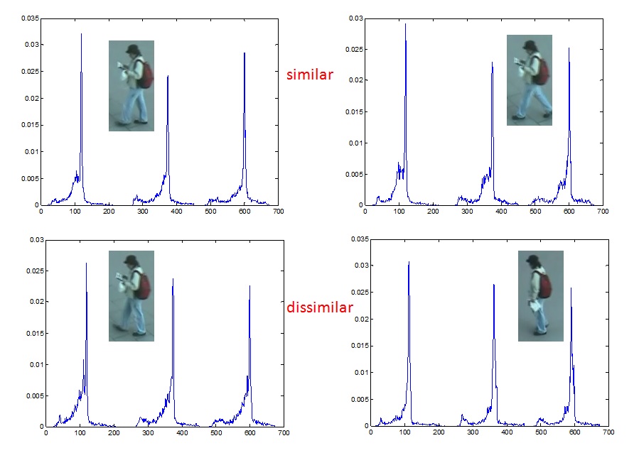
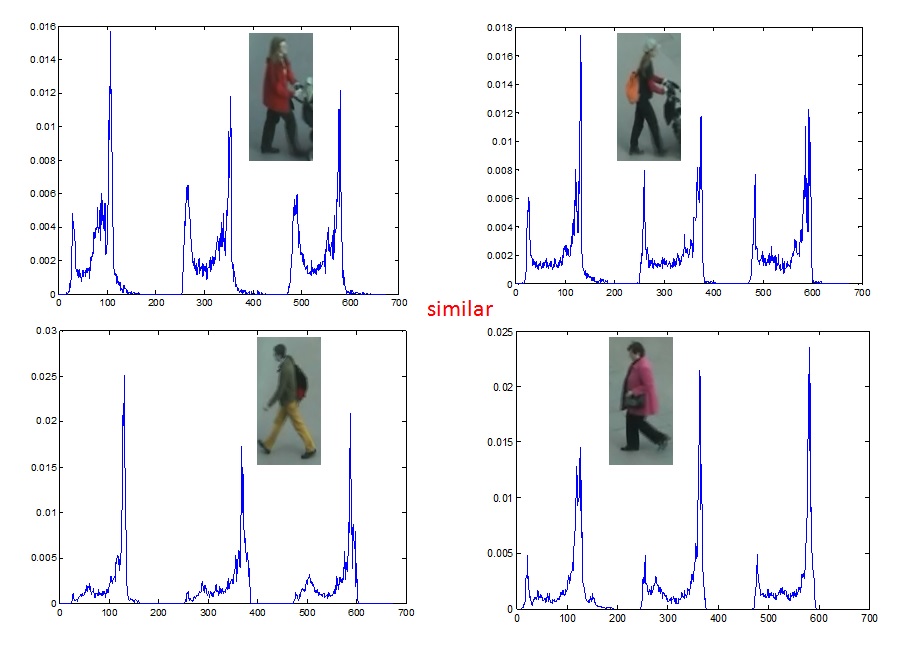
Person re-identification is the task of recognizing individuals across spatially disjointed cameras, and an important problem for understanding human behavior in areas covered by surveillance cameras.
The spreadsheet of the experiment is here.
The results of this experiment is here.
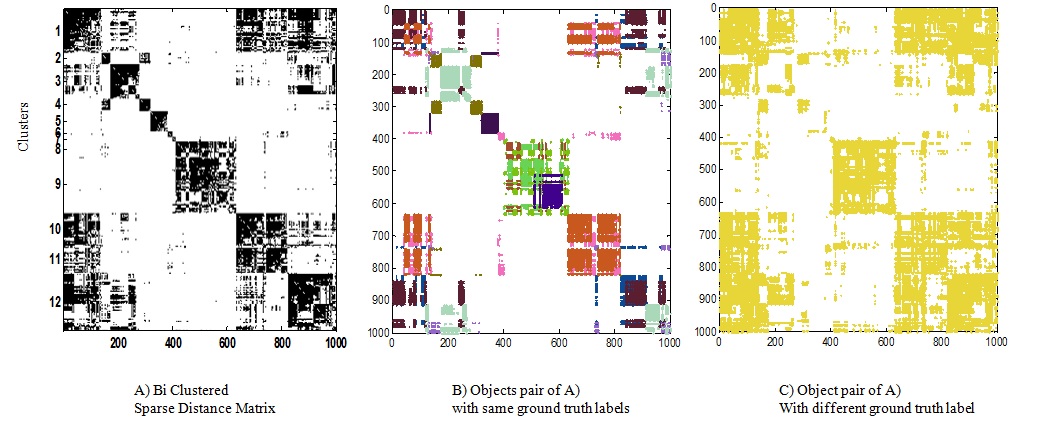
Given the all-pair distance matrix,
- an example k-means algorithm implementation is here.
- an example DBSCAN algorithm implementation is here.
- an example Spectral Clustering algorithm implementation is here.
An example TADPole code with all parameters set, and sample data is available here.
[1] Goldberger, A. L. et al. Physiobank, Physiotoolkit, and Physionet Components of A New Research Resource for Complex Physiologic Signals. Circulation, 101(23), e215-e220, 2000.
[2] Saeed, M., et al. Multiparameter Intelligent Monitoring in Intensive Care II (MIMIC-II): A Public-access Intensive Care Unit Database. Critical care medicine, 39(5), 952, 2011.
[3] Hirzer, Martin, et al. Person Re-identification by Descriptive and Discriminative Classification. Image Analysis. Springer Berlin Heidelberg, pp. 91-102, 2011.
[4] Dhillon, I. S. Co-clustering documents and words using bipartite spectral graph partitioning,ACM SIGKDD, 2001.